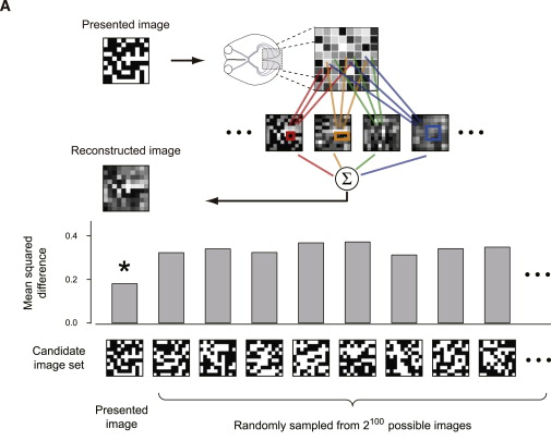
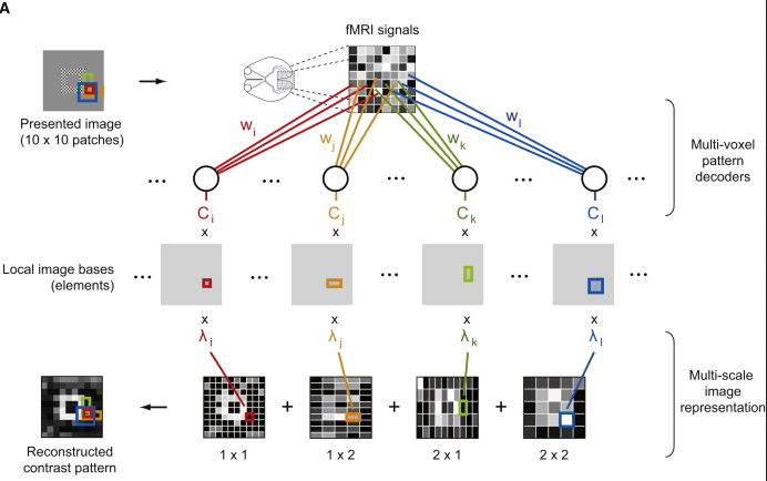
        #Importing required libraries and dataset
        import numpy as np
        from nilearn.input_data import MultiNiftiMasker
        from sklearn.linear_model import OrthogonalMatchingPursuit as OMP
        from sklearn.feature_selection import f_classif, SelectKBest
        from sklearn.pipeline import Pipeline
        from sklearn.metrics import (accuracy_score, precision_score, recall_score, f1_score)
        from matplotlib import pyplot as plt
        from nilearn.plotting import show
        from nilearn import datasets

        #Fetching the Dataset
        miyawaki_dataset = datasets.fetch_miyawaki2008()

        X_random = miyawaki_dataset.func[12:]
        X_figure = miyawaki_dataset.func[:12]
        y_random = miyawaki_dataset.label[12:]
        y_figure = miyawaki_dataset.label[:12]
        y_shape = (10, 10)

        #Load and mask fMRI data
        masker = MultiNiftiMasker(mask_img=miyawaki_dataset.mask, detrend=True, standardize=False)
        masker.fit()
        X_train = masker.transform(X_random)
        X_test = masker.transform(X_figure)

        #We load the visual stimuli from csv files
        y_train = []
        for y in y_random:
            y_train.append(np.reshape(np.loadtxt(y, dtype=np.int, delimiter=','), (-1,) + y_shape, order='F'))

        y_test = []
        for y in y_figure:
            y_test.append(np.reshape(np.loadtxt(y, dtype=np.int, delimiter=','), (-1,) + y_shape, order='F'))

        X_train = np.vstack([x[2:] for x in X_train])
        y_train = np.vstack([y[:-2] for y in y_train]).astype(float)
        X_test = np.vstack([x[2:] for x in X_test])
        y_test = np.vstack([y[:-2] for y in y_test]).astype(float)

        n_pixels = y_train.shape[1]
        n_features = X_train.shape[1]


        def flatten(list_of_2d_array):
            flattened = []
            for array in list_of_2d_array:
                flattened.append(array.ravel())
            return flattened


        #Build the design matrix for multiscale computation
        #Matrix is squared, y_rows == y_cols
        y_cols = y_shape[1]

        #Original data
        design_matrix = np.eye(100)


        #Example of matrix used for multiscale (sum pixels vertically)
        #
        # 0.5 *
        #
        # 1 1 0 0 0 0 0 0 0 0
        # 0 1 1 0 0 0 0 0 0 0
        # 0 0 1 1 0 0 0 0 0 0
        # 0 0 0 1 1 0 0 0 0 0
        # 0 0 0 0 1 1 0 0 0 0
        # 0 0 0 0 0 1 1 0 0 0
        # 0 0 0 0 0 0 1 1 0 0
        # 0 0 0 0 0 0 0 1 1 0
        # 0 0 0 0 0 0 0 0 1 1

        height_tf = (np.eye(y_cols) + np.eye(y_cols, k=1))[:y_cols - 1] * .5
        width_tf = height_tf.T

        yt_tall = [np.dot(height_tf, m) for m in y_train]
        yt_large = [np.dot(m, width_tf) for m in y_train]
        yt_big = [np.dot(height_tf, np.dot(m, width_tf)) for m in y_train]

        #Add it to the training set
        y_train = [np.r_[y.ravel(), t.ravel(), l.ravel(), b.ravel()] for y, t, l, b in zip(y_train, yt_tall, yt_large, yt_big)]

        y_test = np.asarray(flatten(y_test))
        y_train = np.asarray(y_train)

        #Remove rest period
        X_train = X_train[y_train[:, 0] != -1]
        y_train = y_train[y_train[:, 0] != -1]
        X_test = X_test[y_test[:, 0] != -1]
        y_test = y_test[y_test[:, 0] != -1]

        #We define our Prediction function

        #Create as many OMP(OrthogonalMatchingPursuit) as voxels to predict
        clfs = []
        n_clfs = y_train.shape[1]
        for i in range(y_train.shape[1]):
            clf = Pipeline([('selection', SelectKBest(f_classif, 500)),  ('clf', OMP(n_nonzero_coefs=10))])
            clf.fit(X_train, y_train[:, i])
            clfs.append(clf)

        #Run the prediction function

        y_pred = []
        for clf in clfs:
            y_pred.append(clf.predict(X_test))
        y_pred = np.asarray(y_pred).T


        # We need to the multi scale reconstruction
        def split_multi_scale(y, y_shape):
            #Split data into 4 original multi_scale images
            yw, yh = y_shape

            #Index of original image
            split_index = [yw * yh]
            #Index of large image
            split_index.append(split_index[-1] + (yw - 1) * yh)
            #Index of tall image
            split_index.append(split_index[-1] + yw * (yh - 1))
            #Index of big image
            split_index.append(split_index[-1] + (yw - 1) * (yh - 1))

            #We split according to computed indices
            y_preds = np.split(y, split_index, axis=1)

            #y_pred is the original image
            y_pred = y_preds[0]

            #y_pred_tall is the image with 1x2 patch application. We have to make
            #some calculus to get it back in original shape
            height_tf_i = (np.eye(y_cols) + np.eye(y_cols, k=-1))[:, :y_cols - 1] * .5
            height_tf_i.flat[0] = 1
            height_tf_i.flat[-1] = 1
            y_pred_tall = [np.dot(height_tf_i, np.reshape(m, (yw - 1, yh))).flatten()
                           for m in y_preds[1]]
            y_pred_tall = np.asarray(y_pred_tall)

            #y_pred_large is the image with 2x1 patch application. We have to make
            #some calculus to get it back in original shape
            width_tf_i = (np.eye(y_cols) + np.eye(y_cols, k=1))[:y_cols - 1] * .5
            width_tf_i.flat[0] = 1
            width_tf_i.flat[-1] = 1
            y_pred_large = [np.dot(np.reshape(m, (yw, yh - 1)), width_tf_i).flatten()
                            for m in y_preds[2]]
            y_pred_large = np.asarray(y_pred_large)

            #y_pred_big is the image with 2x2 patch application. We use previous
            #matrices to get it back in original shape
            y_pred_big = [np.dot(np.reshape(m, (yw - 1, yh - 1)), width_tf_i)
                          for m in y_preds[3]]
            y_pred_big = [np.dot(height_tf_i, np.reshape(m, (yw - 1, yh))).flatten()
                          for m in y_pred_big]
            y_pred_big = np.asarray(y_pred_big)

            return (y_pred, y_pred_tall, y_pred_large, y_pred_big)


        y_pred, y_pred_tall, y_pred_large, y_pred_big = split_multi_scale(y_pred, y_shape)

        y_pred = (.25 * y_pred + .25 * y_pred_tall + .25 * y_pred_large + .25 * y_pred_big)

        #Check the Scores of the model
        print("Scores")
        print("------")
        print("  - Accuracy (percent): %f" % np.mean([
            accuracy_score(y_test[:, i], y_pred[:, i] > .5) for i in range(100)]))
        print("  - Precision: %f" % np.mean([
            precision_score(y_test[:, i], y_pred[:, i] > .5) for i in range(100)]))
        print("  - Recall: %f" % np.mean([
            recall_score(y_test[:, i], y_pred[:, i] > .5) for i in range(100)]))
        print("  - F1-score: %f" % np.mean([
            f1_score(y_test[:, i], y_pred[:, i] > .5) for i in range(100)]))

        #Finally we plot the Images
        for i in range(6):
            j = 10 * i
            fig = plt.figure()
            sp1 = plt.subplot(131)
            sp1.axis('off')
            plt.title('Stimulus')
            sp2 = plt.subplot(132)
            sp2.axis('off')
            plt.title('Reconstruction')
            sp3 = plt.subplot(133)
            sp3.axis('off')
            plt.title('Binarized')
            sp1.imshow(np.reshape(y_test[j], (10, 10)), cmap=plt.cm.gray,
                       interpolation='nearest'),
            sp2.imshow(np.reshape(y_pred[j], (10, 10)), cmap=plt.cm.gray,
                       interpolation='nearest'),
            sp3.imshow(np.reshape(y_pred[j] > .5, (10, 10)), cmap=plt.cm.gray,
                       interpolation='nearest')

        show()

